Complex Network in Football Clubs and players

Complex Network in Football Clubs and players

When I saw the last blog on cricket world cup's complex network I thought that such kind of networks may be present in many sports one way or other. As football is one of the most famous games in the entire world, I focussed my search on this game and found some interesting information to create a very versatile complex network.

This complex network is based on the football clubs of Brazil and the main focus is on understanding if there exists some complex network properties in them.
Now let us first define out network.

Network: Bipartite network. One side Club and other side Player.

Node: Any player who has ever played in any club.

Edge: If two players have played in the same club, we connect them with an edge going through that club.

Weight of edge: Number of goals scored by a player for a club.

We can immediately see something like the citation netwok here.

Taking the data of 127 clubs and 13,411 players all taken from Brazillian championship from 1971-2002, we can define many statistical features for each club and player. Let G denote the number of goals scored by a club and M denotes the goals conceded then the following graph shows the variation of Nc and G/M follows the Gaussian curve fitting.

Lets try to see the degree distribution of each kind of vertex in the bipartite network. The player probability P(N) show expected decay which happens exponentially. Similar to citation network, N corresponds to the number of clubs a player has been involved in . Club probability distribution was less obvious because of them being in small number.

One thing to notice is that the probability of finding nomadic players is very less as compared to the one stable in one or two clubs.

Now here comes the most interesting part and the best result to showcase in the football network.

We define P(M) as the probability that total of M matches are played by any player (irrespective of the club). There is a kink or elbow in the graph so obtained in the semi log plot and happens at Mc = 40. This is where we can fit the cumulative distribution P(Mc) into two different exponentials.

Pc(M) = 0.150 + 0.857 * 10^(-0.042M) for M <40 and 0.410* 10^(-0.010M) for M>40.

Both of these are shown in  the following figure that the fit the given exponential distribution quite well. One of the most obvious conclusion from the graph is that once a player has found some fame it easier for him to keep playing. But one funny conclusion is that the same applies for player with notoriety. If you cross the threshold Mc, then there is high chance that you have achieved stability in the job as a player. This might be seemingly impractical to say, but we can extend this conclusion to the number of matches a player can survive when suffering from bad form.

Without goals, a football game can never exist. So goals must form most important dynamics of football. Hence the same was plotted with P(G) as the probability of a player scoring G goals. The following graph shows the plot. The cumulative goals scored P(Gc) is also plotted below the P(G) one.

Again an interesting threshold of Gc=10 is found here which separates region in apparently two different regions following separate power laws. Such laws are found many times in scientific collaboration network.

Again the two equations that best fit the network were worked upon and found to follow the following.

Pc(G) = -0.259 + 1.256*G^(-0.500) for G<10

Pc(G) = -0.004 + 4.454*G^(-1.440) for G>10

Also P(G)~G^(-1.5) for G<10

and P(G)~G^(-2.44) for G>10

Using the above graph, of the 11 players in a team, we can easily find which player is supposed to be in what sort of position, like goal keeper,defender or striker. From this distribution we found that nearly two thirds of player forms the less-scoring positions.

Making further attempts to generalise more complex network related features in this field we created a Soccer Player network with making edges between two players present in a team at the same time. This merging is same as that of scientist-paper bipartite network. Out of the obtained graph of 13,411 vertices and 315,566 edges the degree probability P(k) was calculated and average degree was found to be k = 47.1. Also getting the Clustering Coeffiecient of the network gave us

C = 0.79 making it a highly clustered network. The assortavity coeffiecient was A = 0.12 which makes it assortative network although less assortative than that of citation network having A=0.46.

The average shortest path was found to be D=3.29 from which we can logically conclude that there are 3.29 degrees of separation between the players.

An attempt to understand the time based evolution of the network was also made. The results obtained were:

Study on temporal evolution shows the following

1) Increasing mean connectivity k: Player's professional life is turning longer or transfer rate is going up.

2) Clustering Coefficient decreases: Movement of player to some outside club not under study.

3) The network is becoming more assortative with time. This means that segregation of players and transfer between the players in the clubs of similar type.

Conclusion and future works

The study shows that there are many facets in normal life where complex networks can be applied and lead to great predictions once we understand the network. Note that this study was centered around Brazillian clubs. If similar study is promoted for European clubs involving many countries we might get to see good clustering as well as better players to choose for transfer choice among the clubs.

Reference: http://journals.aps.org/pre/pdf/10.1103/PhysRevE.70.037103

Submission By - Nishkarsh Shastri

Analyzing Cricket Strategies using Network Properties

During this World Cup season, it will be interesting to look into a model for analyzing cricket strategies using complex network tools. As we know cricket is a game involving interaction between the two batsmen who are presently batting and between the batsmen and the bowlers. Using partnership data available from crickinfo, we can construct a partnership graph among batsmen within a team and analyze certain properties of this graph to infer the important players in a team, winning strategies for the bowling team, etc.

Measuring the performance of batsmen in a team

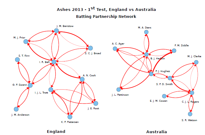
We can generated weighted directed graph for all the players in a team and one such graph per all the teams in a tournament. The weight of a link is equal to the fraction of runs scored by a batsman to the total runs scored in a partnership with another batsman. Thus if two batsmen A and B score n runs between them where the individual contributions are nA and nB, then we draw a directed link of weight nA/n from B to A. Figure 1 shows an example of weighted and directed batting partnership network for two teams - Australia and England in Ashes 2013 test series.

Fig. 1

We use the following centrality scores to measure the individual performance of the players within a team :

• In-strength: For a weighted directed graph, the in-strength s(i)in is defined as 

 where wji is given by the weight of the directed link.

• Page Rank: To quantify the popularity of a player, we use Page Rank as a measure. To begin with, each node is given a uniform probability of 1/N and then using the Page Rank equations, we iterate till a steady state is reached. It is to be noted that the PageRank score of a player depends on the scores of all other players and needs to be evaluated at the same time. The transportation probability q is taken as q=0.15. This choice of q ensures a higher value of PageRank scores. The Page Rank of a player is calculated as: 

• Betweenness Centrality: In cricketing terms, betweenness centrality gives a measure of how the runs scored by a player during a partnership depends on the other player. High betweenness centrality batsmen tend to score runs without loosing his wicket. These batsmen are highly important in a team because their dismissal impacts the network structure. In other aspect, having only a few players with high betweenness centrality indicates an unbalanced team which is highly dependent on a few batsmen. In an ideal case, every team would seek a combination of players where betweenness scores are uniformly distributed among players. The winning strategy for the opponent team would be to get these batsmen out as quickly as possible. 
• Closeness Centrality: It measures how well connected a player is in the team. Batsmen with high closeness centrality tend to be more flexible team players in the sense that they can perform well independent of the changes in batting order according to the game conditions. 

Table below compare the performance of the players for the 1st and 2nd test from Ashes 2013.

As we know these players, we can try to draw conclusions from this table. The betweenness centrality of IR Bell is the highest among all the players. The fact that in the second innings of the first Test at Trent Bridge, he scored 109 when England were 121 for 3 supports this argument. He was able to add 138 runs for the seventh wicket with the tail-ender Broad, and helped England post a target of 311. According to the centrality score IR Bell was the most deserving candidate
for the Player of the match award (Although Mitchell Johnson-4/61 (17 overs) was the man of the match because of his bowling figures which is not captured by this model). Similarly the performance of other players can also be evaluated.

To summarize, this study reveals that network analysis is able to to give a performance score for batsmen in a team. Other than providing a visual summary of the match, partnership graph can be used to measure the popularity and importance of players in a match. Further analysis of the matches in the test series reveals that Australia was highly dependent on the batsmen while England was playing a team-game. By adding additional fields such as "athletic index" of a batsmen and fielding network, we can further capture the difficulty faced by the batsmen while batting.

Reference: Ashes 2013 − A network theory analysis of Cricket strategies, Satyam Mukherjee. 

Chinese Whispers - an Efficient Graph Clustering Algorithm

     Clustering is defined as the task of grouping together objects in such a way that those objects that are similar to each other comes in the same group. The Chinese Whispers algorithm provides a basic yet very effective way to partition the nodes of a graph.

Some to the notations used are as follows:

Let G=(V,E) be a weighted undirected graph with nodes (v_i)∈V and weighted edges (v_i, v_j, w_ij) ∈E with weight w_ij.The degree of a node is the number of edges a node takes part in.The neighborhood of a node v consists of all the nodes that are connected to v.

The Adjacency matrix A_G of a graph G with n nodes is an n×n matrix where the entry a_ij denotes the weight of the edge between v_i and v_j . If no edge exists this weight will be zero.

The Class matrix D_G of a Graph G with n nodes is an n×n matrix where rows represent nodes and columns represent classes (c_i)∈C. The value of d_ij (row i and column j) represents how much v_i belongs to class c_j.

Chinese Whispers Algorithm

The Chinese Whispers Algorithm tries to find out the groups of nodes that broadcast the same message to their neighbors. The algorithm is as follows:

Initialize:
     forall v_i in V: 
          class(v_i)=i;
while changes:
     forall v in V, randomized order:
          class(v)=highest ranked class in neighborhood of v;

The algorithm works as follows in a bottom-up fashion.

Initially all the nodes are assigned to different classes. Then the nodes are processed for a small number of iterations. In each iteration the nodes inherit the strongest class in the local neighborhood. This is the class whose sum of edge weight is maximum to the current node. If there are multiples Strongest class available, one of them is randomly chosen. One important thing to note here is that the classes are updated immediately. This means a node can obtain classes that were introduced in the same iteration. 

                                   Fig 1. Clustering of 11 nodes with CW
                                                        for 2 iterations.


 Formally, the algorithm does not converge. But usually the class do not change after few iterations. The number of iterations depends on the diameter of the graph. Larger the diameter more number of iterations will be required.

Chinese Whispers as Matrix Operations 

     The Chinese Whispers is a special case of Markov-Chain-Clustering(MCL). MCL is the parallel simulation of all possible random walks up to a finite length on a graph G. The idea is that random walkers are more likely to end up in the same cluster where they started than walking across clusters. MCL simulates flow on a graph by repeatedly updating transition probabilities between all nodes, eventually converging to a transition matrix after k steps that can be interpreted as a clustering of G. This is achieved by alternating an expansion step and an inflation step. 
The expansion step is a matrix multiplication of M_G with the current transition matrix. The inflation step is a column-wise non-linear operator that increases the contrast between small and large transition probabilities and normalizes the column- wise sums to 1. The k matrix multiplications of the expansion step of MCL lead to its time-complexity of O(k*n²).



The CW process keeps one single largest entry per row.This leads to drastic optimization possibilities. Let maxrow(.) be an operator that operates row-wise on a matrix and sets all entries of a row to zero except the largest entry, which is set to 1. The algorithm is as follows :

D⁰ = I_n
for t=1 to iterations
     D^t-1 = maxrow(D^t-1)
     D^t = D^t-1A_G
 

 The Time complexity is O(k.|E|). There is a chance the classes might not converge and just oscillate.Fig2 shows an example.

                                    Fig2 : Oscillating States in matrix CW

This is caused due to stepwise update of the class matrix. To avoid this the following measures can be taken:

• Random mutation: with some probability, the maxrow-operator places the 1 for an otherwise unused class.
• Keep class: with some probability, the row is copied from D^t-1 to D^t.
• Continuous update: the classes get updated immediately.
  

Experiments

Bi-partite Clique

    A n-bipartite-clique is a graph of two n-cliques, which are connected such that each node has exactly one edge going to the clique it, does not belong to.

                                         Fig3 : A 10-bipartite clique

  We expect CW algorithm the cut the 2 cliques apart. So the algorithm has 2 choices. Either it can separate it into 2 clusters or combine them into 1 cluster. This is largely dependent on the initial iterations.

                          Fig4 : Percentage of obtaining two clusters when
                                    applying CW on n-bipartite cliques

 From Fig4, We can see that CW algorithm fails on graphs of small size.But this problem does not occur if the graph is large in size.



Conclusion

The Chinese Whispers Algorithm is an efficient Clustering algorithm. This technique seems not to work for graphs of small size. But the main power of CW algorithm lies in Clustering of large graphs in reasonable time. The applications of CW algorithm are enormous. It can be primarily used in NLP.

References

1. C. Biemann. 2006. Chinese whispers - an efficient graph clustering algorithm and its application to natural language processing problems. In proceedings of TextGraphs, 73–80, New York, USA.
2. http://en.wikipedia.org/wiki/Cluster_analysis.

CONFLICTS IN MIDDLE EAST !!!

The Middle East is currently ablaze with a variety of conflicts. A civil war is raging in Syria, in which already hundreds of thousands of people died and millions of people had to flee from their home. On and across those borders, ISIS wages war on both Syrian and Iraqi territory. In Libya the situation has deteriorated into a civil war. Then there is the seemingly never-ending conflict between Israel and Palestine affecting all other conflicts.

All the relationships between these players in the Middle East create a complex web of friendships and enmities. For example, Israel supports an Iraqi Kurdistan, as do the US and the UK. At the same time, NATO ally Turkey is not too happy with an independent Kurdistan. Pakistan is friends with both Saudi Arabia and Syria, while Saudi Arabia positioned itself against Syria. Qatar is also supporting the Syrian opposition similar to Saudi Arabia, but was also supporting the Egyptian Muslim Brotherhood, contrary to Saudi Arabia.

It is rather difficult to make sense out of this intangible web of international relations. Fortunately, the relationships between these countries have been mapped in the following way:

We can understand the conflicts in terms of Power Blocs and Social Balance.

Power Blocs:

In such a scenario  perhaps some power blocs exist, i.e. some groups of countries that are mostly friends, with conflicts running across.From the above network details for each pair of relevant parties whether they are enemies, whether their relationship is strained, or whether they are friends of even allies can be extracted.Now when we use Community detection on the network with respective weights  of -2, -1, 1 and 2 and We use a resolution parameter of 0, which ensures that the average relationship within groups is positive (friendly), while the average relationship between groups is negative (hostile).

When we do this, we obtain the following partition.

The largest cluster consists of the Western countries and regional allies, which surprisingly also contains both Israel and the State of Palestine (and also Fatah). The second largest cluster contains many non-state actors such as Al-Qaeda, Hamas, Islamic Jihad, the Taliban and the Muslim Brotherhood, which seem mostly tied to Qatar as the only state in that cluster. The third cluster groups together well known allies Hezbollah, Iran, Iraq, Russia and Syria. Egypt, Lebanon and Yemen are also clustered together. Finally, both IS and the Islamic Army in Iraq (a Shia militia) are isolated and don’t have any allies.

Note however that this partition is not necessarily always the same, and can differ from run to run (because some parties straddle the boundaries between clusters). Calculating how often the countries end up in the same cluster, we obtain the following figure:

It thus seems that the complex web of relations can thus be reduced to roughly 4 groups (and two isolates), which is a bit easier to understand. Nonetheless, the situation remains quite complex and volatile.Now we look into another concept to understand the situation.

Social Balance.

According to a sociological theory known as social balance, networks tend to become more balanced, meaning that friends tend to share the same friends and enemies, while enemies have different friends and enemies. The idea is similar to the old adage of “the enemy of your enemy is your friend.” There have been various models suggested for how such a social balance may come about. The model followed by (Traag, Van Dooren, De Leenheer, 2013) is described here. The idea here is that parties that have a similar position tend to become friendlier, while those who differ become more hostile. We can also do this for the network here, and let it run until it converges (actually, it goes to infinity, but the sign of the matrix converges, but these are technical details). The dynamics of the process look like this:

Here, the x-axis denotes the time, while the y-axis is the value of the relationship for each pair of countries (which starts out at -2, -1, 0, 1 or 2). The lines are coloured according to their final sign: blue for positive and red for negative. Notice that, even though some relationships start out positive, they may become negative, and vice-versa, some relationships start out negative but may become positive over time. It can be prooved that these dynamics (almost) always converges to a so-called balanced state: it can be neatly divided into two groups, where both groups are hostile towards each other, but friendly towards their own group. A warning is in order, before the results are over-interpreted: it is not known whether these models are predictive or not.

The first group contains most of the non-state actors, including Al-Qaeda, Hamas, Hezbollah, Islamic Army in Iraq, Islamic Jihad, Islamic State, Muslim Brotherhood and the Taliban, which would be supported by Iran, Iraq, Pakistan, Russia, Qatar, Syria and Yemen. The other group would consist of the Western countries and the other Arab states. This is not the most optimistic perspective, since a concerted conflict between these two groups would be devastating. But we shouldn’t draw too many conclusions from this analysis. There are still many uncertainties, and results may differ for slight deviations in the initial conditions. We’ve just used relatively arbitrary weights for constructing this network. Also, the assessment of the relations may not be accurate, and they are definitely not up to date. Finally, I re-iterate, there is nothing yet known about whether this model (or other models) are actually predictive. We should therefore research these models and questions more. Nonetheless, we may obtain some insight by analysing the Middle East relationships from this perspective. Although it may seem unrealistic, let’s keep up hopes that the situation improves.

References

Traag, Vincent Antonio, Paul Van Dooren, and Patrick De Leenheer. 2013. “Dynamical Models Explaining Social Balance and Evolution of Cooperation.” PLOS ONE 8 (4): e60063. 

Traag, V. A., P. Van Dooren, and Y. Nesterov. 2011. “Narrow Scope for Resolution-Limit-Free Community Detection.” Physical Review E 84 (1): 016114

Small Worlds Of Human Language

Language is “one of the wonders of the natural world” and “what makes us human” .Human language can also be modeled and analyzed with complex networks. The conception of language as a system is one of the central assumptions of modern linguistics Human language allows the construction of a virtually infinite range of combinations from a limited set of basic units.

Zipf's Law

Zipf's law states that given some corpus of natural language utterances, the frequency of any word is inversely proportional to its rank in the frequency table. Thus the most frequent word will occur approximately twice as often as the second most frequent word, three times as often as the third most frequent word, etc.

 But many a times such a relation with word frequency often comes to little use.For e.g if the text is scrambled the frequency remains same but it makes no sense.


Information is organized into sentences that are made by words in interaction with each other. Words interact in many ways. Some words co-occur with certain words at much higher probability.
A lexicon is a catalogue of a language's words (its wordstock); and the grammar, a system of rules which allow for the combination of those words into meaningful sentences.

The Word Co-occurrence Graph

It is quite obvious that many co-occurrences occur due to syntactical relationships between words. Links can be formed between words that have  significant co-occurrences in the same sentence. The biggest connected component that results from the basic and the improved methods is called the Unrestricted Word Network(UNW) and Restricted Word Network(RWN).


The figure below shows the degree distribution curve for British National Corpus. They decay with average exponent γ = -2.7 . This exponent in second regime is similar to BA model (γ = -3). The BA model leads to scale-free distributions using preferential attachment.

Degree distribution of UWN(filled circles) and RWN(open circles)

Further the word networks have Small-World features. The average minimum distance between vertices is 2.6 and clustering coefficient is

Connectivity distribution of 5000 most connected vertices in RWN.
The exponent of power tail is nearly 3 indicating preferential attachment 

0.687 which is much higher than that of corresponding random expectation. This result has significant impact because any word during communication can be reached within very few steps.

Some of the studies about the lexical networks that have small world characteristics show that it is polysemy(many possible meanings for a word) and homophony (two words of different origin but have identical pronunciation) .

Two things can be derived if the small-world property holds-

1. Existence of words that speed up navigation to other words. They're called particles and have no semantic value e.g. articles, prepositions etc
2. The existence of brain disorders characterized by navigation deficits in which such words are involved e.g Agrammatism. 

Language Clustering with Word Co-occurrences

Statistics from different languages show that the word co-occurrence network and its syntactic dependent network (two words connected if they're syntactically dependent) are highly similar in terms of network topology. So a word co-occurrence network can substitute a potential syntactic dependency network in studies of linguistic networks.

Clustering of 14 word co-occurrence networks with
eight complex network parameters

Running network algorithms on the same text in a parallel language(as a substitute for syntactic  dependency networks) can help us in clustering languages. This work done by HaiTao and CONG Jin in 2012. They've constructed 14 word co-occurrence networks based on parallel text of 12 Slavic languages and 2 non-Slavic languages and conducted network analysis to them according to different combinations of major complex network parameters. They're able to distinguish Slavic and non-Slavic groups and also group some of slavic languages in their respective sub-branches. The clustering has also captured the genetic relationships of some of these Slavic languages within their

sub-branches.

References

http://complex.upf.es/~ricard/SWPRS.pdf
http://en.wikipedia.org/wiki/Zipf's_law
http://en.wikipedia.org/wiki/Lexicon
http://download.springer.com/static/pdf/877/art%253A10.1007%252Fs11434-013-5711-8.pdf?auth66=1425661617_0c9ab52bec4efb188b5aaa4874f44abc&ext=.pdf
http://arxiv.org/pdf/cs/0701135.pdf