Saturday, April 11, 2015

Cupid in your network


Single and secretly wondering which of your friends might be able to introduce you to your future soulmate?

Sociologists have long studied the dating pool problem, noting that an acquaintance is more likely to introduce you to your mate [1] than a close friend is. Your close friends tend to know all of the same people as you, while acquaintances have greater “bridging social capital,” connecting you to diverse clusters of new people. On the other hand, your close friends might be more motivated to set you up; they care more about your happiness, and they know you better. So who, really, is more likely to set you up? And do these “matchmakers” have special characteristics that make them ideally suited to the task? (Note that when we say “matchmaker” we mean “a friend who introduced you” rather than a professional.)

To answer these questions, a survey was done of approximately 1500 English speakers around the world who had listed a relationship on their profile at least one year ago but no more than two years, asking them how they met their partner and who introduced them (if anyone) and then analyzed network properties of couples and their matchmakers using de-identified, aggregated data.

What does a typical matchmaker looks like?

Unlike the stereotype of an older woman from Fiddler on the Roof, our matchmakers looked pretty similar to the couples they were matching. They were young (most often in their 20s, as were most of the survey respondents), half of them were men, and roughly half of them were single (much like most of the future couple's other friends). So you might not be able to identify your cupid at a glance.

However, our matchmakers had a secret weapon: more unconnected friends. To start, matchmakers have far more friends than the people they're setting up. Before the relationship began, the people who later got matched had an average of 459 friends each, while matchmakers had 73% more friends (794 on average). This isn't that surprising, because network science tells us that your friends usually have more friends than you do [2] . But even compared to the couples' other friends, matchmakers have 8% more friends. So they're unusually well-connected.


Matchmakers have 73% more friends than the typical person they set up.

But more than simple friend count, what matters is whether matchmakers' networks have a different structure. And indeed, they do. Though they have more friends, their networks are less dense: their friends are less likely to know each other. We measure this with the clustering coefficient [3], which is 6% lower for matchmakers than other friends of the couple. Matchmakers also have 4% more isolated nodes as a proportion of their network, or people who have no other mutual friends. Matchmakers typically have about 16 unconnected ties in their networks, and each one is an opportunity: people who both know the matchmaker, but don't yet know each other.

 
A typical matchmaker's graph has a lot of nodes but relatively few triangles (people with another friend in common). Each pair of unconnected nodes is an opportunity for an introduction.

Are matchmakers close friends or acquaintances?

Matchmakers were pretty close friends to the people they later introduced. (Makes you wonder why they didn't introduce their friends sooner!) More than half of the survey respondents said they felt “very” or “extremely” close to the matchmaker before the match was made. Nearly half spoke to the matchmaker every day, and two thirds spoke to their matchmaker more than once a week. And half had known the matchmaker for three years or more, as did their future partner. So by every measure, matchmakers were close friends with the future couple.

 
Matchmakers were more likely to be close friends, rather than acquaintances.

However, survey responses are clouded by retrospective bias. Wouldn't you grow closer over time to the person who introduced you to your partner? And that rosy haze can make it hard to remember how close you really felt two years ago. So, for that an examination was done on the network data from the time before the relationship to see if people were actually close to their matchmaker  and then counted the number of mutual friends each person in the couple had with the matchmaker before the relationship started, a common proxy for relationship closeness. Matchmakers typically had 57 friends in common with either person in the future couple, amounting to about 6% of their pool of friends. Does that make them close friends? One good comparison point is the couple today: they typically have 52 friends in common, or about 7% of their pool of friends. If romantic partners are your gold standard for close friends, the matchmakers look like strong ties!

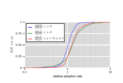
Notably, the fraction of mutual friends between the matchmaker and a member of the couple is significantly higher when they are of the same gender, around 7.4% when the relationship started compared to only 5.1% when they are of the opposite gender.

Couples who met through a friend vs. those who met another way: How do their networks differ?

Couples who were introduced by a friend are more likely to have at least one friend in common a year prior to the start of their relationship (84% of them) compared to those who met in other ways (74% only), which is to be expected – this quantity increases over time, and a few months into the relationship, more than 99% of couples have a friend in common, regardless of how they met.
More interesting though, is that the fraction of mutual friends starts higher for couples who were *not* introduced by a mutual friend (around 4.4% overlap 18 months prior to the start of the relationship) compared to those who were (about 3.4% at that time). It is notable that that quantity increases faster for the latter, to the point that 18 months into the relationship the overlap of social networks of both members of the couple averages at around 7.7% whether or not they were introduced by a friend.

We can understand this by the fact that matchmakers act as bridges between communities or social groups: when you meet someone at school or at work, both you and the other person evolve in the same social circles, hence you have a higher overlap. But imagine one of your friends introduced you to someone at a different school; you might have fewer friends in common with that person at first, but over time you both start making new friends in each other's schools.

 
Couples who were introduced by a friend had a smaller fraction of mutual friends prior to the relationship.

If no one introduced them, how did people meet their partner?

Couples who found each other without a friend introducing them most often met at school. But nearly 1 out of 5 couples met through an online dating service or app. Keep in mind these are primarily couples in their twenties and thirties who started dating in 2013 or early 2014.

Fun fact: As many couples met through Facebook as at a party or in a bar.

This is consistent with a Pew study [4] finding that many social network site users have followed or friended someone because one of their friends suggested they'd want to date that person. And many of our respondents cited Facebook as playing a role in the early stages of their relationships: (Quotes have been edited for length and names have been changed.)

Dan first became interested in me because of a picture he saw of me on facebook. I met the person who introduced me to Dan at a party that was organized on Facebook. Now that I think of it, it's possible that I wouldn't even know Dan if Facebook didn't exist.

We were acquaintances, but after she posted on my wall that we had a lot in common, we began dating.

Without that friend suggestion in his newsfeed, I am not sure he and I would be together today!

 
People most often met their partner at school. As many couples met through Facebook as met at a party or bar.

References
1. Interpersonal Ties (http://en.wikipedia.org/wiki/Interpersonal_ties)
2. Friendship Paradox (http://en.wikipedia.org/wiki/Friendship_paradox)
3. Clustering Coefficient (http://en.wikipedia.org/wiki/Clustering_coefficient#Local_clustering_coefficient)
4. Pew Study (http://www.pewinternet.org/files/old-media//Files/Questionnaire/2013/Survey%20Questions_Online%20Dating.pdf)

Wednesday, April 8, 2015

How do I become a Twitter Stud ?

Today,Twitter is one of the most trending OSN. People are crazy for popularity on twitter. Do you post your tweet and keep endlessly waiting whether some of your friend/family will retweet it and it will give you an adrenaline rush ? Believe me,Deep down your heart even you do that ! So,The questions is How do I become popular on twitter ? This is a two step process - The first step being following massive number of people.Many of them will follow you back because of the "Follow back syndrome" .Once you have enough number of followers,it's time for some math. ( You might wish to  unfollow few of the people who trusted you and followed you back! Thanks to twitter,it doesn't show unfollow notifications)


The second step being increasing the visibility of your tweets. To increase the visibility of your tweets,you would like to mention few users in your tweet which you think would retweet it.Now,the question is How do we select the users ??

  • The user must be popular. duh! 
  • The users are active on twitter while you want to post the tweet
  • The users have a good history of retweeting
  • The users are susceptible of being interested in the tweet
Here are few statistics on the tweet proportion v/s number of retweets for different number of mentions.


Now,the following picture shows us this mention-dependency of top 10 trending hashtags .It seems that highly popular hashtags are heavily dependent on mention links.

```


Several users can be mentioned in a tweet, however this number is limited as the tweet should be less than 140 characters. This problems thus leads to finding the right features evaluating these three components and the trade-off between them.What if we assign a utility score to each user and map them to a knapsack problem ? 

The knapsack problem with the following constraints.
Total Budget : 140 - number of characters in the message(m).
Value of the user : S(u,m) ( This my friend is the utility score which we calculate for user u based on his popularity and the expected probability of retweeting m)
Weight of user : Number of characters in his name + 2 ( Well,one for @ and one for space between multiple users)
This problem will return the set of users which we will mention in our tweet.

Okay,Knapsack is defined.Brace yourselves! Here comes the most important part,the utility score for a user.

This score is the product of three functions that respectively evaluates the Popularity of the user to
mention, its Activity and its Interest to the message. 
The score is given by: S(u, m) = f (u) * pow(g(u),α) *pow(f (u, m), β ) 

where 

f(u) = the number of followers of u.
g(u) = the number of retweets made recently by u
f(u, m) = the similarity of the message m to the last messages of u.(Standard NLP techniques used )

Obviously,now is the time for Twitter's beautifully made Twitter API! Sadly,there are few constraints within a 15 minutes window.
  • get 5000 followers (resp. friends) of a user: 15 requests.
  • get the basic information of a user (particularly its number of followers): 180 requests.
  • get the 200 last tweets of a user: 180 requests.
So,the algorithm goes as follows :
  • Crawl the followers wishing to tweet the message m.
  • Select the friends of the user which are not his followers and among these users select randomly 180 users
  • For each of these 180 users u, crawl its number of followers and set the value of f(u), crawl its 200 last tweets and compute g(u) and f(u, m) out of it
  • Now that the S(u,m) is calculated for all users,Solve the knapsack problem defined above and return the set of users.
Now,Tweet the message m followed by a newline character and the screen names of the users selected, each one preceded by the character @ and separated by spaces. (Now realized why did we do a +2 in the knapsack problem ?? )

After one day the tweets of the users mentioned are crawled to check which users retweeted. The coefficients α and β are then updated taking all available data to improve the utility score.

Increasing the visibility of your tweets will have a higher chance of retweets. More the retweets,more viral your tweet,more viral you and voila,you're a twitter stud!

Please follow me on twitter for further updates. ( See what I did there ?)

References :


  1.  An empirical approach towards an efficient “whom to mention?” Twitter app
  2. Adrien Guille, Hakim Hacid, Cecile Favre, and Djamel A Zighed. Information diffusion in online social networks: A survey. ACM SIGMOD Record, 42(1):17–28, 2013
  3. Kyumin Lee, Jalal Mahmud, Jilin Chen, Michelle Zhou, and Jeffrey Nichols. Who will retweet this? In Proceedings of the 19th international conference on Intelligent User Interfaces, pages 247–256. ACM, 2014.


Monday, April 6, 2015

Diseases and Protein Protein interactions

To understand the molecular basis of genetic diseases, it is important to discover their causal genes. Typically, a disease is associated with a linkage interval on the chromosome if single nucleotide polymorphism (SNPs) in the interval are correlated with an increased susceptibility to the disease. These linkage intervals define a set of candidate disease-causing genes. Genes related to the same disease are also known to have protein products that physically interact A class of computational approaches have recently been proposed that exploit these two sources of information—physical interaction networks and linkage intervals—to predict associations between genes and diseases. Methods typically begin with an artificial disease subinterval and test how well they can identify a known causal gene from among a fixed number of nearby genes in the query subinterval. In another stringent method instead of ranking only genes in the subinterval, all genes in all intervals related to a query disease are ranked.  This more stringent approach is advantageous because it allows us to find disease-causing genes that lie in existing disease intervals but that were previously not associated with the disease. Consequently, we can gauge a gene's relatedness to any query disease.

Network-based algorithms to predict gene–disease associations:


A widely used network-based approach (‘Neighborhood’) predicts for a protein p the annotations that are associated with more than θ percent of p's network neighbors. The method associates a gene with a disease if it lies within a linkage interval associated with the disease and interacts with ≥1 gene annotated with the disease.


Random walks have been used to transfer annotations within networks. We define a random walk (‘RW’) starting from genes known to be associated with a query disease d. At each time step, the walk has a probability r of returning to the initial nodes. Once the process converged (L2-distance between probability vectors in consecutive time steps <10−6), a prediction was made for all genes in relevant intervals with visitation probability greater than θ.


Graph partitioning is a promising technique for predicting gene–disease associations because it can uncover functional modules in PPI networks, and phenotypically similar diseases are often caused by proteins that have similar biological processes. Three graph partitioning algorithms were recently shown to find the most biologically relevant modules: GS, MCL and VI-Cut. GS1 losslessly compresses the input network, producing a smaller summary network and a list of corrections to over-generalizations in the summary. The nodes in this summary correspond to modules in the input network. The summary graph can be further compressed by discarding the list of corrections and applying GS again, resulting in larger modules (‘GS2’). This process can be repeated i times, yielding a ‘GSi’ method. The ‘GS-All’ method makes the union of the predictions made by GS1, GS2 and GS3. VI-Cut is a semi-supervised clustering method that uses annotations in the training set when creating modules.


Quality of Network based predictions:


In a typical implementation the following results were obtained:


The random walk methods and Prop show a clear dominance over the clustering and neighborhood methods. The clustering methods, VI-Cut, and GS1 and its variants GS2, GS3 and GS-All, which have not previously been appraised for the task of predicting gene–disease associations, performed slightly worse than the random walk methods, but better than the neighborhood approaches. They achieve between 18.4% and 68.6% precision and 1.1% and 17.9% recall.


Conclusion:


The classes of network-based methods considered here each approached the task of predicting gene–disease associations using very different philosophies. Although random walk approaches are superior to clustering and neighborhood approaches. In general certain diseases for which high-throughput PPI networks were an especially useful source from which to make high-quality predictions can be found. Diseases that have little correlation with the interaction network call for higher quality networks or an integrative approach that considers sequence, functional annotations, expression data or other additional information.


References:


Aerts Set al. Gene prioritization through genomic data fusion. Nat. Biotechnol. 2006

  1. Brohee S
  2. van Helden J. 
Evaluation of clustering algorithms for protein-protein interaction networksBMC Bioinformatics 2006

  1. Fraser HB
  2. Plotkin JB
Using protein complexes to predict phenotypic effects of gene mutationGenome Biol. 2007

  • Ideker T
  • Sharan R
  • Protein networks in diseaseGenome Res. 2008


    Friday, March 27, 2015

    Time Constrained Networks

    One of the key features of complex networks is that they capture interactions which have no limitations.  In most electronic systems, be they Facebook, emails or web pages, we can make connections across the world with little if any cost.
    However what if there are constraints on the links made in a network? Surely we should change the way we study networks if space, time or some other constraint is having a significant effect on the formation or use of the network.  This has been a major interest of researchers over the last few years. Space is one obvious limitation as in some cases long distance are less likely to be made. There has been a lot of work in this area over many decades.
    It is only more recently that the role of time in networks has began to receive more attention. A lot of this recent interest in how to deal with networks where the connections, are made at one time.  That is because most communication networks, emails, phone calls and so forth, are of this type.
    Yet networks are made of two parts: vertices and edges. The recent work is focussed on the case where it is the vertices, not the edges, which are created at a definite time. In such temporal vertex networks, causality forces the interactions between nodes to always point in one direction. For example consider a citation network formed by academic papers. The nodes in our network are the academic papers and the links are formed by their bibliographies.  So if paper A refers to another paper B then we can be (almost) sure that A was written after B. Information can therefore flow only from B to A. In fact any set of documents can only refer to older ones such networks are common. In law, judges refer to previous judgments to support their arguments.  When registering a patent, prior art needs to be cited, that is other previously granted work which may have some relevance to the current claim.
    The same types of structure occur in several other situations.  Any situation where there is a logical flow has the same causal structure.  If we have a project where the nodes represent individual tasks then an edge from task S to task T could represent the fact that task T requires task S to have been completed before task T is started.  This has been the focus of work on temporal vertex networks in computer science. The logical flow of a mathematical argument or an excel spreadsheet show the same properties.  These networks define what is called a partially ordered set or poset and it is under this title that one finds relevant work coming from mathematicians. A final example comes from the Causal Sets approach to quantum gravity.  Here space-time is discrete not continuous, and these discrete points are the nodes of the network.  The nodes are connected by edges only if they are causally connected and causality again gives these a common direction.
    All of these temporal vertex networks have a key property.  That is they contain no loops if you always follow the direction on the edges.  You can not go backwards in time. Thus the traditional name for such a network is a directed acyclic networks or DAG for short.
    So the question is how can we adapt traditional network measures to deal with the fact that these networks, DAGs, are constrained by causality?  Are there new measures we should employ which give more insights to such networks?
    One feature of a DAG we have been exploiting is that if we always follow the direction of the arrows, the direction of time, then not all nodes are connected. If we like we could add edges whenever there is such a path connected a late node to an earlier one, a process known as transitive completion.  On the other hand we could remove as many edges as we can while leaving the causal relationships intact, a process known as transitive reduction. That is, if there is a path between two nodes in the network before transitive reduction, then there will still be a link afterwards.

    Image result for time constrained networks
    Example of the transitive reduction (left) and the transitive completion (right) of the directed acyclic graph in the centre.
    What we have done (in Transitive Reduction of Citation Networks) is look at how real data from citation networks behaves after transitive reduction.  We find that different types of citation network behave very differently. The citation network formed from academic papers taken from the arXiv repository and the network of US Supreme Court judgments both show that about 80% of the edges are not needed to retain all the causal relationships.  On the other hand the patents network shows the opposite behaviour with all but 15% of edges being essential. The edges removed tend to be the citation to older papers. One interpretation is that academics and and judges may be citing well known early papers and judgments though their current work is only directly related to more recent documents. Perhaps some of these citations do not indicate the early work was needed but reflect other motivations, such as simple copying of popular papers or review in the field which at best only have general relevance.
    The number of citations to a document after transitive reduction certainly gives us a different view of the importance of different documents. For instance paper hep-th/9802109 on the arXiv (Gauge Theory Correlators from Non-Critical String Theory by Gubsner et al.) was cited by 1641 papers in the network, but only three citations remained after TR! On the other hand, paper hep-th/9905111 (Large N Field Theories, String Theory and Gravity by Aharony et al.) has also large number of citations in the raw data, 806, yet after transitive reduction it has 77, so retaining far more of its original citations. Perhaps information in the second paper was used more diversely.
    We can find similar examples in the US Supreme Court citation network. The case Schneider vs. New Jersey (1939)’ has 144 citations in the original data but this drops to just just one after transitive reduction. Stromberg vs. California (1931) also falls from 132 citations to just one. Conversely, the case Heller vs. New York (1973) only shows a slight fall after transitive reduction, falling from from 68 to 48 citations and has the most citations in our reduced network. The second most cited case after transitive reduction is Hamling vs. United States, which drops from 68 to 38 citations. Wikipedia lists hundreds of Supreme Court cases but the last two are not famous enough to make the Wikipedia list. The analysis suggests they may have more importance than a simple citation count would suggest. At the very least it might be be worth checking out documents that are highly cited in the essential.
    Another way to look at citation networks is to see if we can define a dimension to the network.  That is we can try to quantify how much variation there is in the citation process.  A low dimension means that there are few directions , few distinct themes relevant for citation in a document.  A high dimension indicates that there is a wide range of relevant but distinct directions from which a document will draw on for inspiration.  We were often able to assign an interesting value for the dimension of our citation data.  For academic papers, we found that different fields of research have different dimensions.  For papers in the hep-th arXiv section (largely string theory) we generally find a low dimension of around 2 while for theoretical papers closely linked to particle physics experiments we find more variation as indicated by a higher dimension of 3. The quant-ph also around 3 while the astro-ph section had a slightly higher dimension of around 3.5. So clearly despite similarities in the main data using standard measures, our time-aware dimension measures show clear differences in the citation behaviour of different areas. String theory in particular seems to be a tightly knit collection of work with each work largely dependent on all the other work, few independent directions can be pursued. The US Supreme Court judgments were more complicated.  Small samples (usually from modern judgments) showed a dimension of around 2.5 to 3 but larger samples, typically ranging from modern to the earliest judgments, had lower dimensions, closer to 2. We interpreted this as reflecting the way that there were few early judgments compared to the number produced to day.  So that the further back we traced in time to find the influence of judgments on recent ones, the smaller the variation.  Perhaps that is not so surprising and we might expect a similar shape if we could follow scientific papers back to the 18th century! patents on the other hand showed a much higher dimension though again these were involved.
    It is clear from just the few studies we have made that time makes a crucial difference to the structure of a network. There is surely much more to find when networks are embedded in time.

    References:

    Clough, J. R.; Gollings, J.; Loach, T. V. & Evans, T. S., Transitive Reduction of Citation Networks, J.Complex 
    Dowker, F. Causal sets as discrete spacetime, 2006. Contemporary Physics, 47, 1-9
    Holme, P. & Saramäki, J. 2012. Temporal Networks Physics Reports, 519, 97-125
    Simkin M.V. and Roychowdhury V.P., 2003. Read before you cite! Complex Systems 14 269-274

    Social and temporal properties of Apps

    Apps are important part of everyone’s lives. They exhibit a rich temporal structure of user adoption and long-term engagement. Also social ecosystem helps in driving the adoption and engagement of apps.
    In the first part we will discuss the social properties of apps and how user’s probability of adopting an app depends both on properties of the local network structure and on the match between the user’s attributes, his or her friends’ attributes, and the dominant attributes within the app’s user population. In the second part we will develop a retention model that represents a user’s tendency to return to an app.

    We would like to place apps in a low-dimensional space that can provide a view for how they are distributed across the social network of users. To do this, we begin with two basic definitions

    •  We say that the popularity of an app, denoted p(x), is the probability that an individual selected uniformly at random from Facebook’s population is a user of the app.
    • We say that the sociality of the app, denoted p(x|y), is the probability that a member of Facebook is a user of the app given that they have at least one friend using the app.

    Studying the distributions of p(x) and p(x|y), and how they are jointly distributed across apps, allows us to ask a number of questions. In particular, how socially clustered is the app? And how does it depend on the type of app, or characteristics of the app’s users?
    Moreover, p(x|y) can in principle be high even when p(x) is low -- this would correspond to an app that is popular in a focused set of friendship circles, but not on Facebook more broadly. On the other hand, if p(x|y) is not much more than p(x), then it says that users of the app are spread out through the social network almost as though each member of Facebook independently flipped a coin of bias p(x) in order to decide whether to become a user of the app -- there would be no effect of the social network at all.

    Figure 1: App sociality. Top left: Horizontal axis is app popularity, and vertical axis is the relative increase in adoption likelihood for people who have friends who also use the app. Right panels: Horizontal axis is app popularity, vertical axis is app sociality. The colors represent the number of apps falling within the given bin. The labeled colors indicate the relative frequencies of observations in each bin, such that the lowest values have been normalized to 1.

    We see in Figure 1 that the apps fill out a wedge-shaped region in the p(x)-p(x|y) plane.  If the social network had no relationship to app usage, we would see the diagonally sloping line p(x) = p(x|y); in the plot this corresponds to a line that lies slightly below the diagonal lower boundary of the points in the heat map. Thus, there exists a frontier in the space of apps that is almost completely asocial — those apps that lie parallel to this diagonal line — but essentially no apps actually reach the line; even the most asocial apps exhibit some social clustering. We see this in the approximately horizontal top boundary of the points in the heat map — this is a frontier in the space of apps where knowing that a person x has a friend using the app gives you a fixed probability that x uses it, independent of the app’s overall popularity on Facebook. The wedge-shaped region in a sense has to come to a point on the right-hand side, as p(x) becomes very large: once an app is extremely popular, there is no way to avoid having pairs of friends using it almost by sheer force of numbers. And given the crowding of app users into the network, there is also no way for the extent of social clustering to become significantly larger than one would see by chance.


    For each app, we consider everyone on Facebook who has friends using the app, but who has not used the app themselves by time t.


    Figure 2: Relationship between national identity of potential app adopters, that of their current user friends, and the likelihood of their adopting the app. Blue: Relative adoption rates when a potential user and their current user friend are from the majority to when potential user is in majority and current user friend is in minority. Green: Relative rates when potential user and current user friend are in same minority to when potential user is in minority and current user friend is in majority. Red: Relative rates for when potential user and current user friend are in same minority to when they are in different minorities. The blue curve indicates that when a potential user is from the majority country, their current user friend could be from either the majority or a minority and they are still equally likely to adopt an app more often as less. In contrast, when the potential user is from a minority country, in 75% of apps they adopt more frequently when their current user friend is from the same country as them.

    Consider a Facebook user A who does not currently use the app, and suppose that has exactly one friend B who uses the app (that is, A has between 1 and 5000 friends on Facebook, but for our purposes here, exactly one of those friends is an app user). We choose some attribute on users (for example nationality, or age); we let f(A) and f(B) denote the value of this attribute for A and B, and we let f* denote the modal (or median) value of the attribute across all app users.

    Suppose that A is different from the typical user in this attribute, in the sense that f(A) not equal to f*. Is A more likely to adopt the app if the friend B is similar to A, or if B is similar to the typical app user? We now say that a(i, j) is the adoption probability of a user A who has one friend B using the app, with f(A) = i and f(B) = j. (Note that f* = 0 according to our notation, since 0 is the most prevalent nationality in the app.) a(i, i)/a(i, 0) > 1, indicating a clear aggregate tendency for the question in the previous paragraph: a user A is more likely to adopt the app in general when A’s one friend using the app is similar to A, not to the typical app user. In contrast, when f(A) = f* , the ratio a(0, 0)/a(0, i) is balanced around 1, so there is no clear tendency in adoption probabilities between the case f(B) = f* and f(B) not equal to f* : for users who have the modal attribute value, the attribute value of their friend does not have a comparably strong effect.


    Figure 3: The probability that a user adopts the app given that they have one friend using the app. as a function of (left) the friend’s age offset from the median and (right) the user’s age offset from the median. The left plot indicates no apparent relationship between the age of the friend and that the user adopts. In contrast, the right plot illustrates that young users and users who are aged between 10 and 30 years above the median age are more likely to adopt. Users who are more than 40 years older than the median age are less likely to adopt. The probabilities were binned by age into 20 equally populated bins and the reported adoption probabilities are bootstrap estimates. The thick central line is the median bootstrap estimate of the mean, while the three outer bands indicate the 68%, 95%, and 99.7% confidence-intervals.


    For an app to have long term success we expect that it needs to maintain a relatively high level of user retention. We would like to have a model of retention that characterizes not only whether an individual will log into the app the very next day, but for any day subsequent to their first login.
    We start with the population of newly installed users, n(0), and assume that at every time step each user has a constant probability of leaving, x0. This mechanism gives rise to exponential decay:
    dn(t)/dt = - x0n(t) → n(t) = n(0) exp(−x0 t),
    where n(t) is the number of app users at time t. It turns out that this model does not yield a good fit to the data. However, the fit improves if we introduce a second parameter to the model by fitting from the second day; that is, we fit both for the decay rate, x0 , and the fraction of users that returned on day 2. With this relaxation from fitting day 1, the model becomes
    n(t) = An(0) exp(−x0 t).
    It is interesting that the exponential decay model fits the day 2 and onward trend well while not fitting day 1: it is reasonable to expect that there is a discontinuous transition in the probability of returning given an install versus an install and a return the following day. Day 1 users are dominated by those who use the app exactly once, whereas all the other days contain a signal from users who exhibited at least some level of continued interest in the app

    There are a number of further aspects of the app ecosystem that would be interesting to take into account in future work. First, app adoption is driven in part by the marketing and other recruitment strategies of the app owners. Although our models incorporate the numbers of new users coming to the app over time, they do not differentiate between organic growth and advertising-driven growth. Furthermore, it is not clear whether sociality of apps might accelerate growth or decline or both. Finally, it is unclear whether some features might be early harbingers of future behavior, e.g. whether the change in retention of long-time or recently acquired users is more useful in forecasting the eventual adoption of the app.

    References:


    http://arxiv.org/abs/1503.06870 : The Lifecycles of Apps in a Social Ecosystem – [ Isabel Kloumann, Lada Adamic, Jon Kleinberg, Shaomei Wu]